Sea-ice conditions in the first half of October 2019
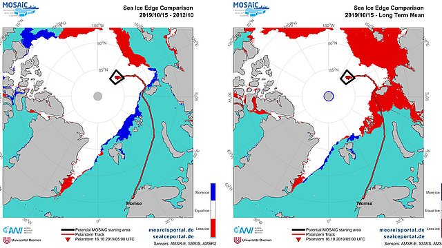
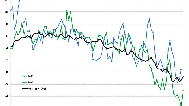
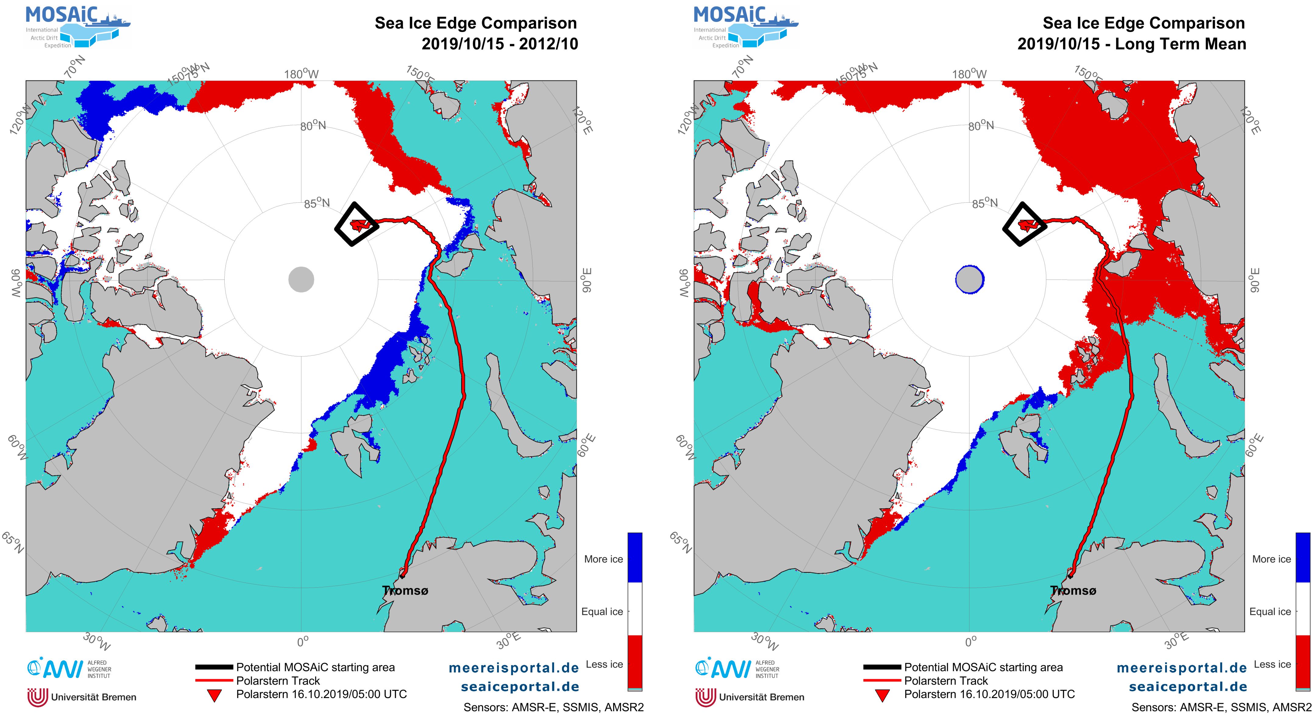
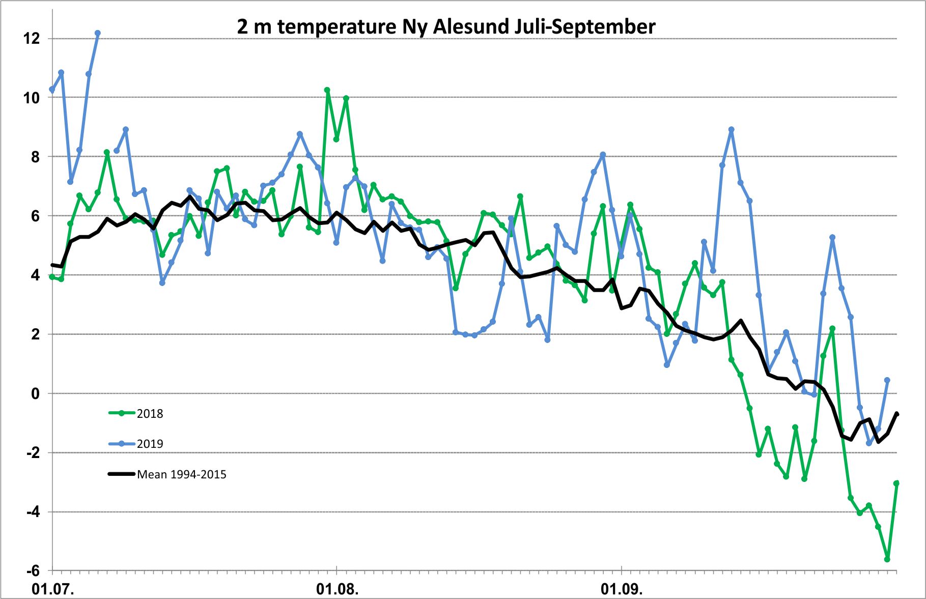
In mid-September, the autumnal sea-ice formation process began in the western Arctic Ocean (see Figure 1). Sea ice extent is with 4.97 Mio. km² far below the long-term average of this time of the year. That being said, the month of October is setting new records: the sea-ice cover has never been so low at this time of year. If we look at the maps comparing the sea-ice extents in 2012 and the long-term average, we can see that, especially to the north of the Laptev Sea and East Siberian Sea and spanning to the Beaufort Sea, many regions now contain much less sea ice than they normally do in October (see Figure 2). In terms of assessing this situation, the measurements taken in the extended vicinity of RV Polarstern during the MOSAiC expedition, which revealed a great deal of thin, rotten ice, are especially interesting. The current situation can most likely be attributed to two major processes: first of all, temperatures continue to be very mild in the Arctic, and large quantities of warm, moist air are being transported to the region from the Pacific and Atlantic alike. In this regard, the first half of October was remarkable; the warmer conditions can be clearly seen, e.g. at the AWIPEV research station on Spitsbergen (see Figure 3). The second major cause: the ocean is uncharacteristically warm for October, and is cooling only slowly, thanks to the warm atmosphere (see Figure 7). Both the water and air are still very warm, and are expected to stay that way for the remainder of the month.
Looking back on September 2019
Looking back on the summer of 2019 in the Arctic, we can say that it was unusually warm and characterised by frequent inflows of warm air from northern Siberia and the Bering Strait (for more information, click here). The effects could be seen in the significant loss of Arctic sea ice and the continuation of the negative long-term trend.
In September, the mean sea-ice extent was 3.97 million km² (see Figure 4), the second lowest since the beginning of satellite observation; in 2012 the mean extent was ca. 480,000 km² lower. In comparison to the long-term average for 1981-2010, the 2019 extent was 2.48 million km² lower. The minimum sea-ice extent was reached on 15 September 2019 and, at 3.77 million km², was the second lowest ever recorded. Afterwards, the sea ice above all rebounded in the northern Beaufort Sea, Chukchi Sea, eastern Siberia and the eastern Laptev Sea. In addition, sea-ice growth was observed near the Canadian Arctic Archipelago and to the northwest of Greenland, although part of the sea ice made its way to the northeast of Greenland thanks to drift. At the same time, warm southerlies produced a retreat of the ice margin in the western Laptev Sea and the Kara Sea. The Northeast Passage was still open at the end of September (source: NSIDC). In comparison to the minimum year 2012, the ice extent in the Barents, Kara and Beaufort Seas was greater than in 2012, although it was lower in the Laptev Sea (Figure 5) – the northern sector of which is home to the starting area for the MOSAiC expedition. This aspect was particularly critical for the beginning of the drift experiment, since much of the ice encountered was too thin.
The data on the sea-ice extent reveals a clear trend, with an average decline of ca. 0.8 million km² per decade since 1979 (see Figure 6). That being said, a considerable degree of variability in the change rates also becomes apparent when, instead of a 41-year-long timeframe, the focus is placed on the individual decades. For example, the period 1990 – 2000 could be interpreted as a stagnation of the sea-ice retreat in summer; the same is true for the years 2007 – 2016. Yet this period also included the years with the third lowest (2007) and lowest ever (2012) sea-ice extent. This illustrates the difficulty of making quantitative statements on the change rate for a highly variable system and on an inter-annual time scale like that used for the sea-ice extent. Accordingly, it makes better sense to focus on long-term variations on a decadal time scale, and on the basis of time series that are more than 30 years long, than to compare the inter-annual variability.
Generally speaking, September was dominated by warm temperatures. The atmospheric temperatures over the ocean at 925 hPa (ca. 750 m above sea level) were 2 to 4 degrees Celsius higher than the temperatures in the reference period (1981-2010). The maximum difference of 4°C was reached over the Beaufort Sea, north of Alaska. The surrounding landmasses reached temperatures that were 1-2 °C above the mean temperature in Eurasia, while the temperatures in northern Canada and Alaska were 1-4 °C above the long-term average. The greatest deviations were in Yukon and eastern Alaska. An exception to the rule: southern Greenland, where the temperatures were 1°C below those in the reference period on average (Figure 7). Nevertheless, Greenland, too, experienced a particularly intense melting season this year, during which nearly 60% of its surface was subjected to melting processes in August. What effect this will have on the overall loss of mass for Greenland’s inland ice is something we’ll only be able to assess in the course of the next several months. The loss of mass in Greenland this summer has already surpassed 400 Gt of ice, which is comparable to that in 2010, but falls short of the greatest loss to date, in 2012.
The MOSAiC expedition has found the ideal ice floe for its drift experiment
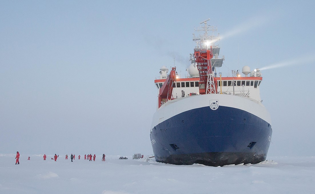
On 20 September 2019, the MOSAiC expedition departed from the port of Trömsø! In our sea ice ticker, we reported on the ship’s progress twice a week. In the meantime the RV Polarstern has found a suitable ice floe, on which the research camp will be erected and a ‘distributed network’ of measuring and monitoring stations will be set up in a 40-km radius around the ship. To aid in the search for the ideal floe, Russian and German sea-ice experts alike engaged in helicopter flights to scout the area; in a second step, ice cores were drilled and other tests were conducted on the most promising floes to gauge their thickness and other characteristics.
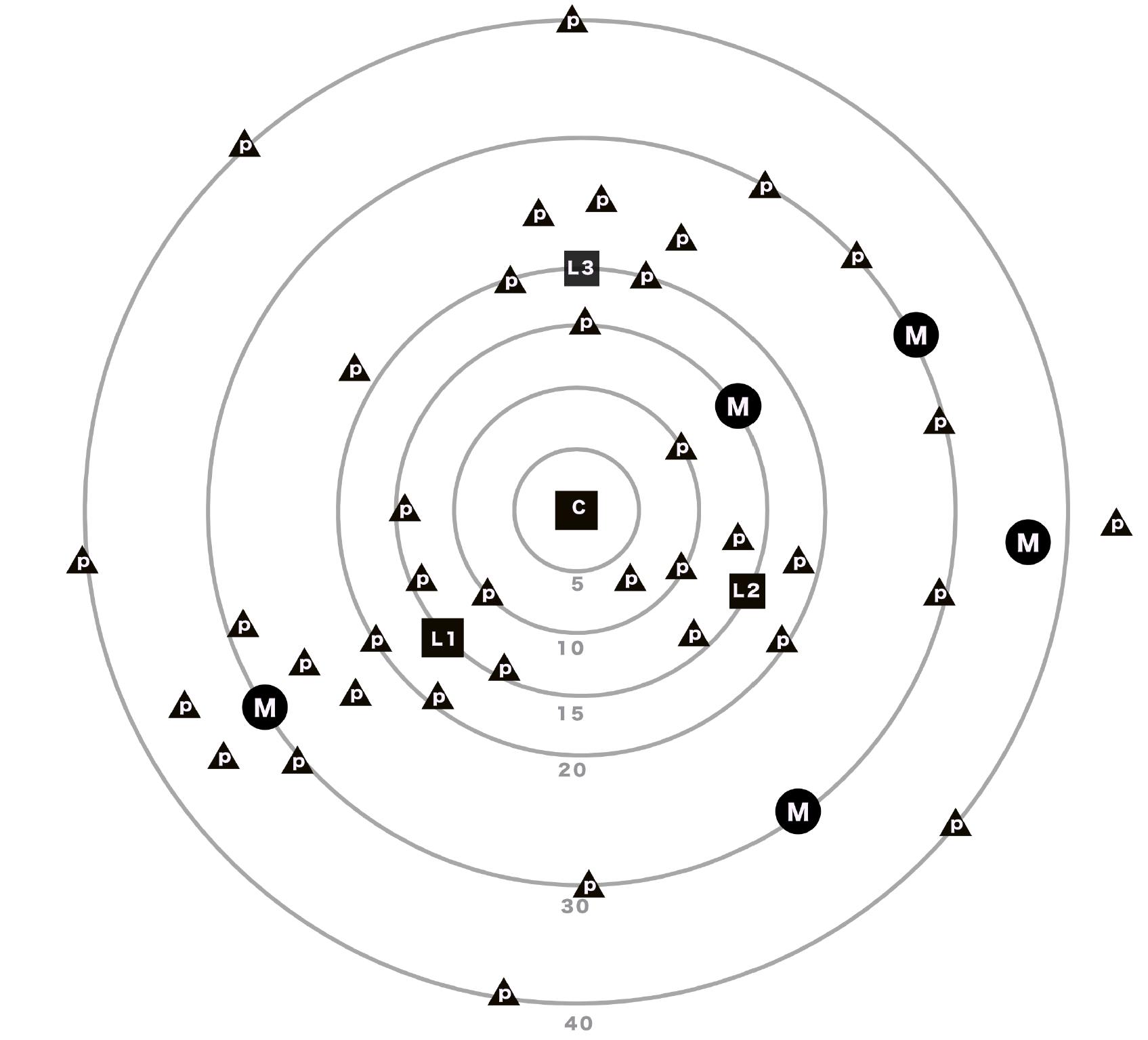
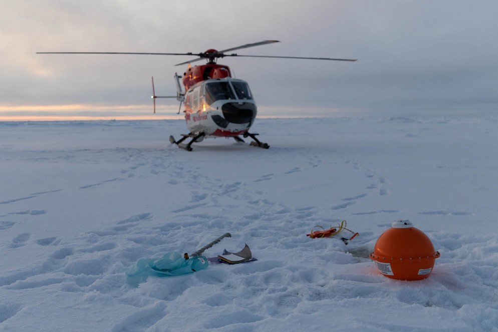
Figure 9 shows the monitoring network, spread out in a 40-km radius around RV Polarstern (C) and consisting of various sensors and buoys (Figure 10). Dr Robert Ricker, a sea-ice physicist at the Alfred Wegener Institute in Bremerhaven, provided support for the efforts to find the ideal floe by preparing detailed analyses of the satellite data, which he sent from Bremerhaven. From February 2020, Ricker himself will join the 3rd leg of the expedition. He describes the current ice conditions as follows: “The summer melting in 2019 not only produced a major decline in sea-ice extent, but also a substantial reduction in ice thickness, especially in MOSAiC’s starting area. As a result, it was difficult to find suitable floes that could serve as the basis for the research camp and the ‘distributed network.’ But thanks to a focused survey of the vicinity, which combined satellite images, helicopter flights, and gathering core samples on the floes themselves, a number of candidate floes were quickly identified.”
Contacts
- Dr. Robert Ricker (AWI)
- Dr Renate Treffeisen (AWI)
- Dr Klaus Grosfeld (AWI)
Questions?
Contact us via E-Mail or our contact form.
Graphics


