Measurements In the Snow and Ice
Taken together, spaceborne (from satellites) and airborne measurements (from aeroplanes and helicopters) offer a very good scientific representation of the sea-ice cover’s current status. Yet the picture isn’t complete without measurements taken at the micro-scale – that is, on the surface of the ice itself. Only then can small details – like the structure of the snow and ice – be recognised, which have a tremendous influence on important functional parameters like heat transfer between the ocean, ice and atmosphere, or the ice’s ability to reflect sunlight (albedo). Researchers can use this data e.g. to improve sea-ice simulations and to make sea-ice forecasts more reliable. Last but not least, taking measurements on the ice’s surface is not just necessary; it’s also an unforgettable experience for all polar researchers, putting them in direct contact with a habitat that is vital to our planet’s future climate. In this section, we’ll introduce you to the most important tools that they use while working on the ice.
Why are snow measurements so important?
The snow cover on sea ice is an important component in the climate system of the polar regions and significantly affects interactions between the atmosphere, sea ice and ocean. Due to its albedo, snow is essential to the surface energy balance and determines how much incoming solar radiation is reflected, absorbed, or passes through the snow into the ice and ocean. As such, the snow is also an early-warning system of sorts for the underlying sea ice: intensifying warming first affects the snow’s characteristics, before reaching the sea ice below it.
In this regard, it is also important to understand that the snow behaves quite differently on Arctic sea ice than on Antarctic sea ice: while the surface of the snow on Arctic sea ice is subject to pronounced seasonality and melts completely in summer, the snow on Antarctic pack ice only exhibits very low melting rates in the course of the seasons. Rather than melting, this snow changes its physical characteristics through e.g. various melting and freezing cycles, and therefore makes a key contribution to the sea-ice mass balance in the Southern Ocean.
In addition to its direct influence on the ice’s physical characteristics, snow can make it more difficult to measure and interpret geophysical parameters like sea-ice thickness and volume using satellite-based remote sensing methods. As a result, e.g. laser altimetry is used to determine the snow’s freeboard. In order to translate freeboard into ice thickness, precise assumptions regarding the snow thickness are called for. This is especially true for Antarctic sea ice, since it is characterised by a comparatively high ratio of snow thickness to ice thickness, which significantly affects the freeboard. Accordingly, ice-thickness estimates depend heavily on the freeboard-to-ice-thickness conversion, which can produce considerable uncertainties in thickness estimates for Antarctic sea ice. In addition, the inadequate parametrisation of snow and its characteristics in numerical models leads to major uncertainties in corresponding descriptions of the current sea-ice situation and in sea-ice predictions on larger spatial and temporal scales.
As such, although the snow cover on the sea ice represents an essential variable in the status of the polar climate system, it is also one of the least well-known and most difficult parameters to characterise in the coupled polar climate system – which makes it all the more important that we extensively measure the snow on our expeditions to the Arctic and Antarctic.

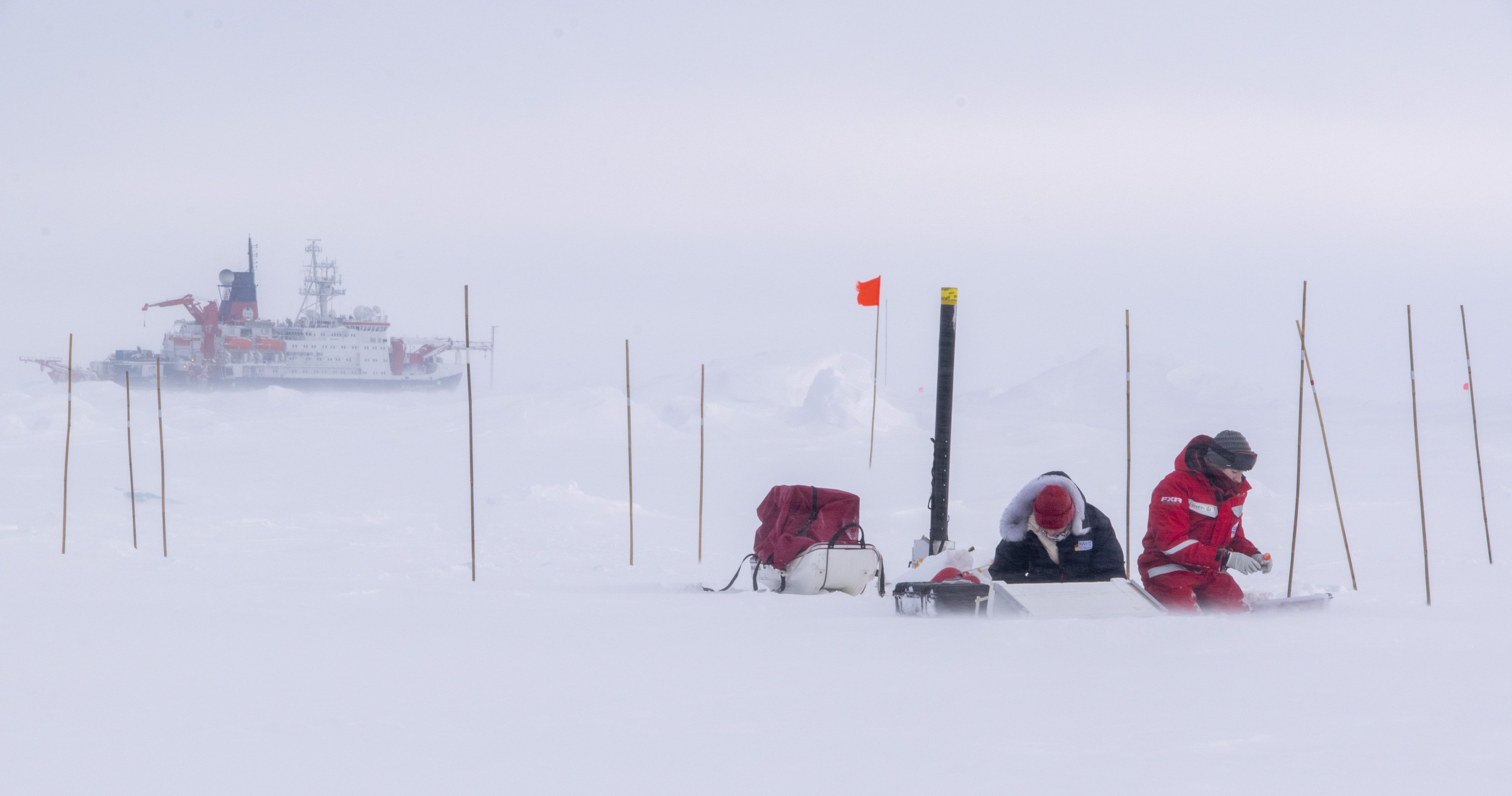
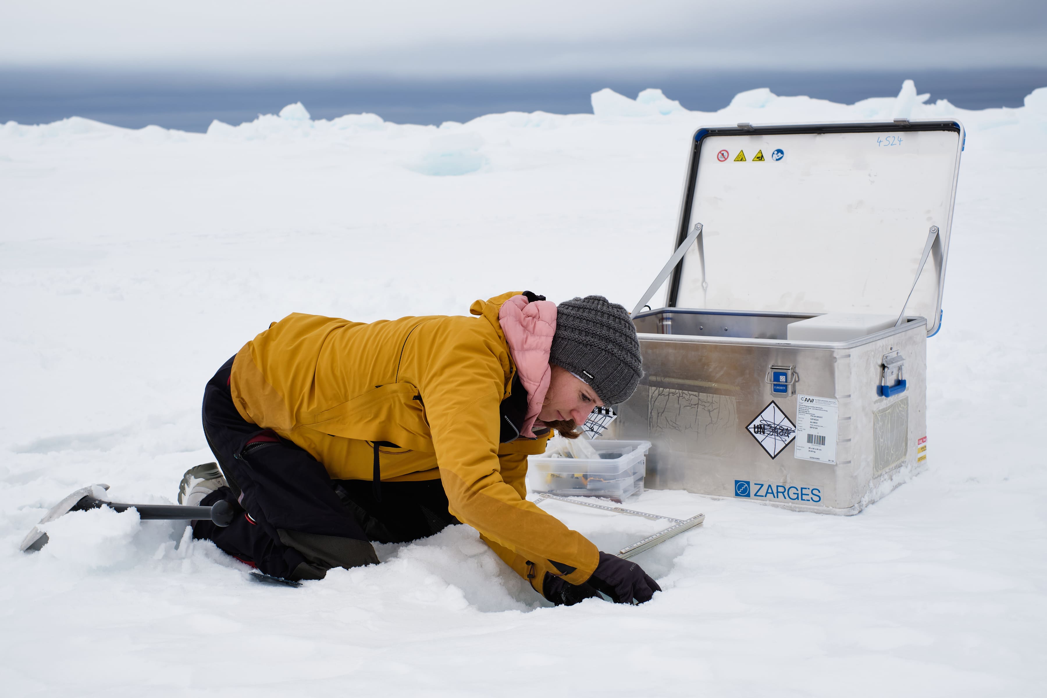
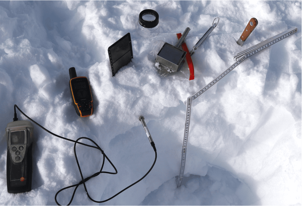
But how can snow characteristics be accurately described? A classic and frequently used manual method is snow-pit analysis. Here, a representative spot is chosen to dig a hole in the snow – from its surface to the sea ice below. Within the newly dug snow pit, the measuring is done on a smooth vertical wall not exposed to direct sunlight.
First, a vertical profile of the snow temperature with a resolution of 2 to 5 cm – depending on the snow thickness – is recorded with the aid of a needle thermometer. Next, what is known as the volumetric snow density is determined – again, through the entire layer of snow. To do so, uniformly sized snow blocks are dug out of the measuring wall and weighed. Combining the volume (a known parameter) and weight allows the density to be calculated. The snow’s mean overall density can be determined in the same way. To do so, a snow block that includes the entire height of the snow is cut out and measured.
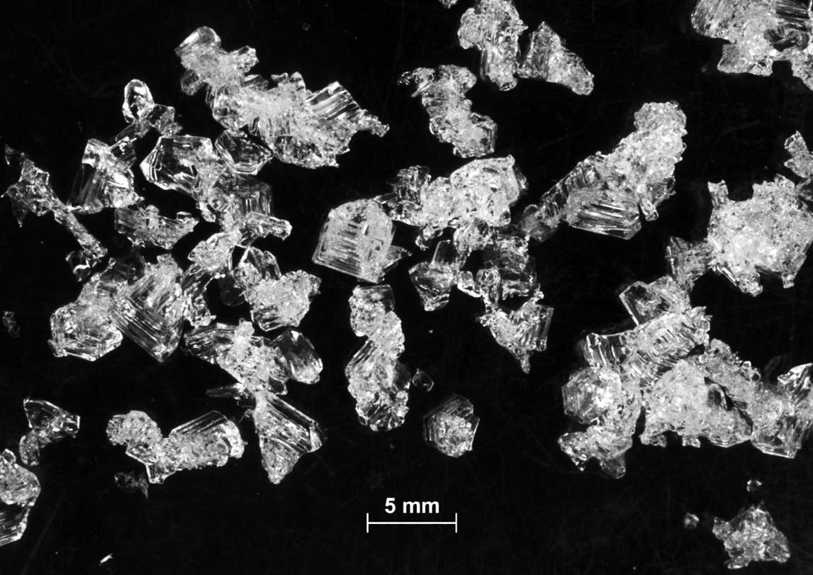
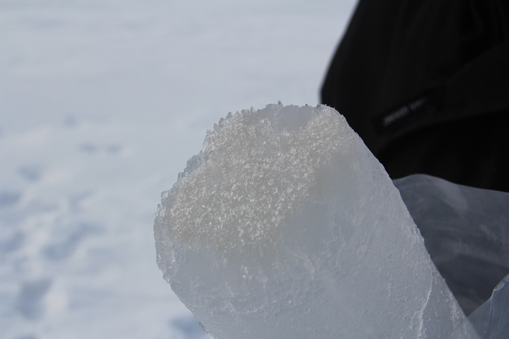
After that, it’s time to get down to the “nitty gritty” – and to (literally) take a much closer look at the snow: to measure the snow stratigraphy, the snow is visually inspected and individual layers are identified. To determine the size and type of snow grains, individual snow crystals are examined with a magnifying glass and millimetre-scale chart. In this way, fragmented crystals can be distinguished from multifaceted crystals, and from the exceptionally large depth hoar crystals. Whereas the latter chiefly form when there are extreme temperature gradients between the warm snow and cold atmosphere, small, round and highly compacted crystals are mostly produced by major wind events in the region. In contrast, the snow hardness can be rated using one of six categories simply by testing it with your hand: can I stick my fist (very soft), 3 or 4 fingers (soft), or only 1 or 2 fingers (moderate) into it? Or do I need a pencil (hard) or knife (very hard)? Or is it actually a layer of ice in the snow? Of course, these characteristics can also be measured in the laboratory using far more technical means, namely computer tomography (CT). Using a CT scan, an extracted grain of snow is continuously analysed, and the results can be used to create a 3D model of the snow cover. However, the machine is very sensitive to shaking or vibration, which prevents it from being used on normal ship-based expeditions in the ice.
In terms of measuring snow wetness, either a dielectric technique can be used – or once again, a faster and more classic method: simply trying to make a snowball out of the snow. While the snow is far too cold and dry in winter and crumbles immediately, in spring this method can be used to check whether the snow has already begun to melt and the percentage of liquid water inside has increased. If it has, it can easily be made into snowballs – having a snowball fight in the name of science; what more can you ask for?


Fierz, C., Armstrong, R. L., and Durand, Y. (2009): International Classification for Seasonal Snow on the Ground, Technical Documents in Hydrology. International Association of Cryospheric Sciences / UNESCO.
As one can easily imagine, manually determining the snow density can be taxing, particularly when it has to be done layer by layer in snow that is up to a metre thick. Since researchers frequently have only a few hours to complete these measurements on the sea ice, as a rule only two or three snow pits can be dug out per floe – and therefore no conclusions can be drawn regarding the spatial variability of snow density on the floe in question.
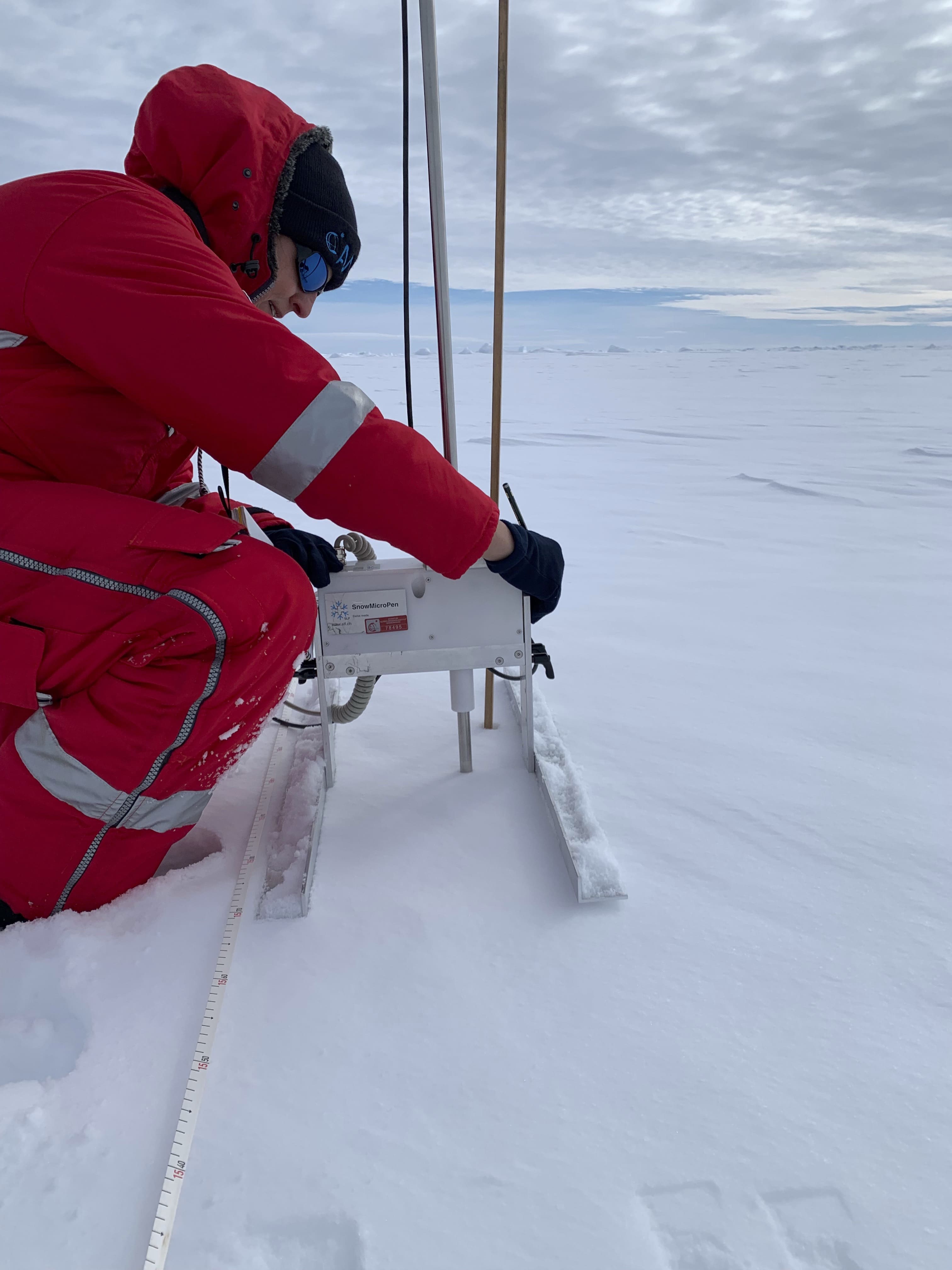
Accordingly, the SnowMicroPen, or SMP for short, is also used. The SMP is a high-resolution snow penetrometer, which can be used to objectively measure the binding forces between the snow grains with high vertical resolution, and to do so quite quickly – in under a minute. Its most obvious feature is a long metal rod, which a motor inserts into the snow at a constant speed. At the end of the rod is a piezoelectric force sensor, which measures the physical resistance as a function of depth. Once the resistance passes a certain threshold, the rod is retracted. When this happens, it means the boundary layer between the snow and sea ice has been reached, i.e., that the snow has been completely penetrated – or that the snow contains thick ice lenses.
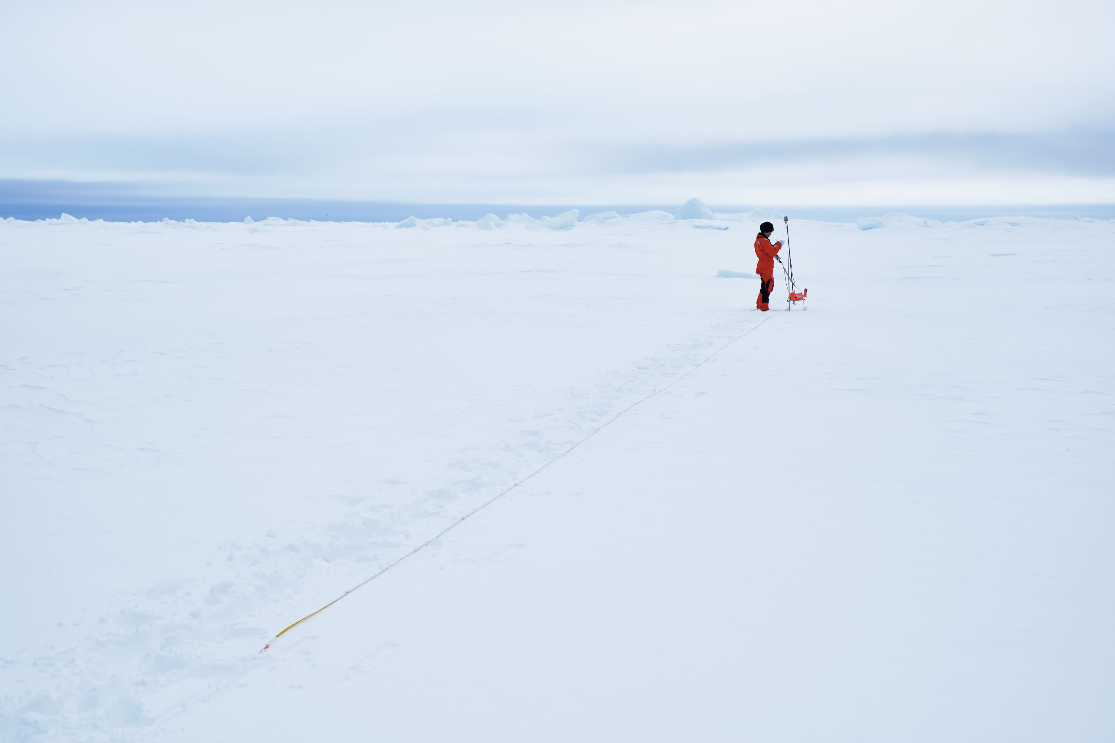
These measurements are often taken along straight profiles (referred to as transects) across the respective ice floe: at a fixed interval between measuring sites, the device is used over 100-metre-long transects.
Back on board the ship, the force readings can be converted into snow thicknesses using simple formulae. The main advantage compared to manual snow-thickness measurements: the SMP delivers high-resolution density profiles, allowing individual layers to be identified and / or the density of the entire snow column to be determined – and not at just two or three spots, but in some cases at up to 100 sites per floe. Nevertheless, snow-pit measurements remain a valuable tool: they can help validate the SMP readings, making the calculated snow thicknesses more precise in the process.


Surface topography of sea ice, measured with a terrestrial laser scanner (TLS)
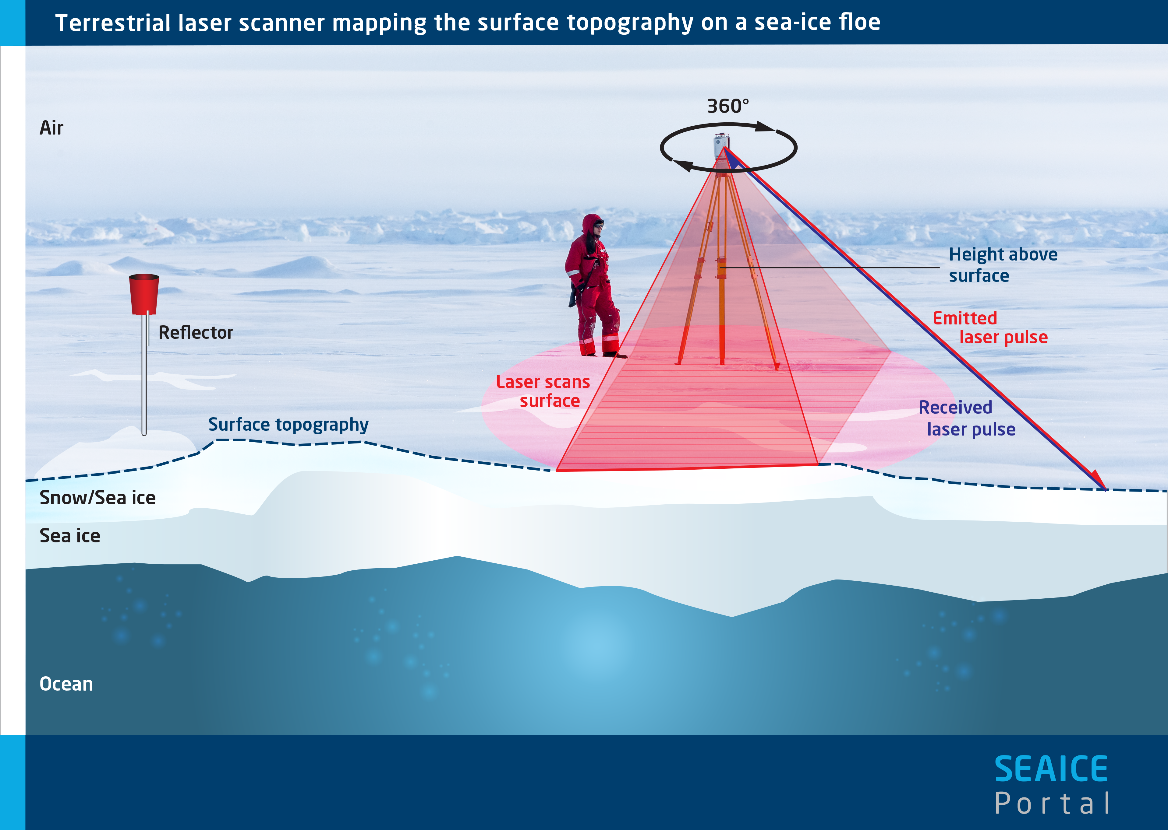
Measuring the spatial distribution and temporal development of the surface topography is essential for investigating the mass balance and energy balance of sea ice. With the aid of a terrestrial laser scanner (TLS, Figure 1), maps of the surface topography with high spatial coverage and resolution can be created.
As a rule, a TLS is mounted on a tripod, ca. 2 metres over the sea-ice surface. Its transmitter emits laser pulses traveling at the speed of light, which are reflected back to its receiver by the sea-ice surface. By measuring the elapsed time between transmitting and receiving the laser pulses, the difference in height and therefore the surface topography relative to the position of the TLS can be determined (using the speed of the pulses in the air). The laser pulses scan the surface in a fan-shaped pattern. In addition, the TLS rotates 360° while taking a reading, allowing it to survey the surface of a larger area. Various measuring stations, referred to as scan positions, are distributed throughout the target area. With the aid of reflectors installed in said area, a single software package can be used to combine the data from all stations in order to create a complete terrain model.
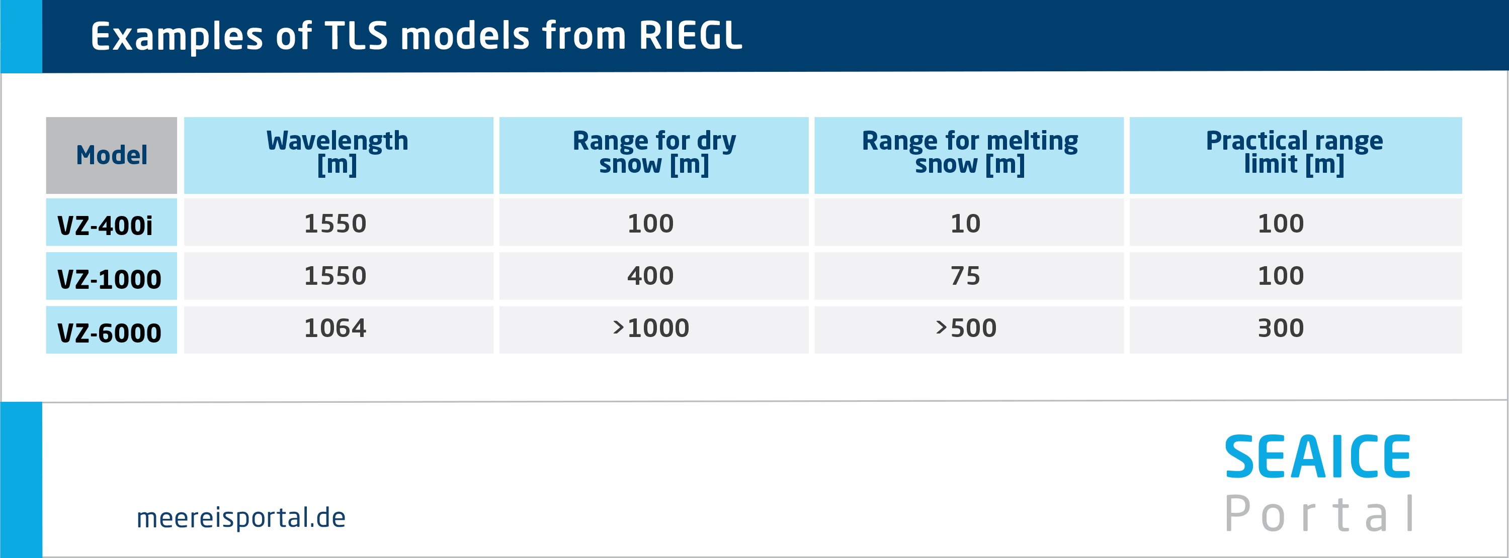
The TLS devices currently in use have a variety of ranges, which depend on the laser power, laser wavelength, and the local surface and snow conditions (s. Table). In practice, the maximum range of a given TLS is also limited by the current visibility. At distances of more than ca. 300 metres, even on relatively smooth ice the shading effect becomes too pronounced due to the low angle of incidence for the laser light. Due to their powerful lasers, some TLS models can e.g. be harmful for the eyes and have to be used with care.
The results of a TLS scan include the surface reflectance (Figure 2A), the height of the surface relative to that of the TLS (Figure 2B), and the distance from the TLS. The reflectance describes how much optical input (here: from the laser) is reflected back by a given material (here: the sea ice) at a certain wavelength. In this regard, the reflectance of water – e.g. in melt ponds (Figure 2A, B) – or of wet snow is very low.
In addition to measuring the surface topography and changes in it (e.g. due to snow accumulation or snow melting), other important parameters for sea-ice research can be deduced. These include the distribution and abundance of melt ponds (e.g. Anhaus et al., 2021a, Figure 2A); the formation, evolution and draining of melt ponds (Polashenski et al., 2012), and the height of the snow cover. The latter is only possible when the scans are made on level sea ice with a constant thickness within the ice-thickness measuring device’s measurement uncertainty, as the change in height then only results from the change in snow cover. (Anhaus et al., 2021b). In addition, the positions of other instruments installed on the sea ice, and the distances between them and the TLS, can be validated. In this way, various measurements can be compared with one another. Moreover, TLS readings can be used to add spatial information and coordinates to aerial photographs of the ice’s surface (geo-referencing, e.g. Anhaus et al., 2021a).
Anhaus, P., Katlein, C., Nicolaus, M., Arndt, S., Jutila, A., & Haas, C. (2021b). Snow Depth Retrieval on Arctic Sea Ice Using Under-Ice Hyperspectral Radiation Measurements. Frontiers in Earth Science, 9. doi:10.3389/feart.2021.711306
Anhaus, P., Katlein, C., Nicolaus, M., Hoppmann, M., & Haas, C. (2021a). From Bright Windows to Dark Spots: Snow Cover Controls Melt Pond Optical Properties During Refreezing. Geophysical Research Letters, 48(23). doi:10.1029/2021gl095369
Polashenski, C., Perovich, D. K., & Courville, Z. (2012). The mechanisms of sea ice melt pond formation and evolution. Journal of Geophysical Research: Oceans, 117(C1). doi:10.1029/2011jc007231
Reference data
Representative samples of the data gathered during expeditions to the Arctic Ocean are available hereRepresentative samples of the data gathered during expeditions to the Arctic Ocean are available here:
doi:10.1594/PANGAEA.940151, doi:10.1594/PANGAEA.932593, doi:10.1594/PANGAEA.932597, doi:10.1594/PANGAEA.932598 , doi:10.1594/PANGAEA.932599


