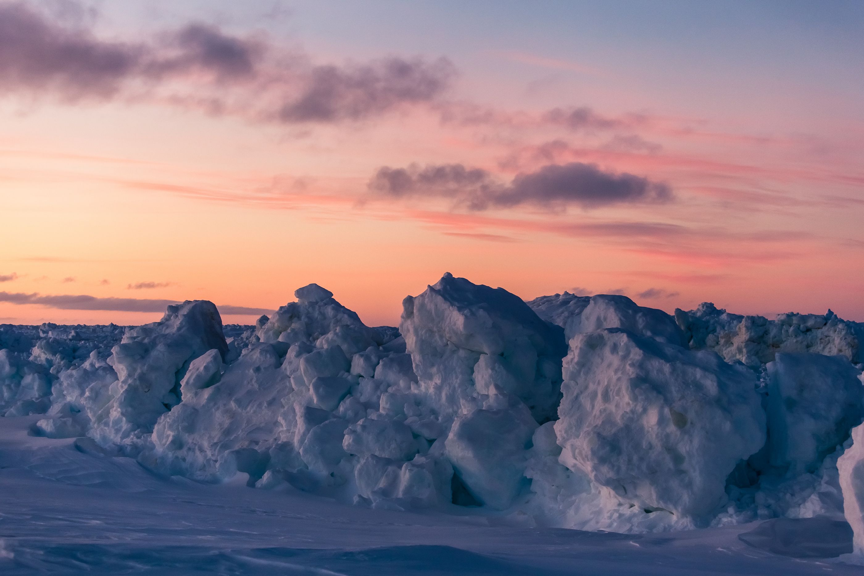
Sea-ice Modelling
In this section of the SEA ICE PORTAL, we’ll provide an overview of how sea ice is simulated in computer models and the scientific questions that sea-ice models can be used to address.
After sea-ice observation, sea-ice modelling is an important tool for investigating the physical basis of sea-ice development and, in the process, arriving at a better understanding of the ice’s interactions with the atmosphere and ocean, as well as the causes of changes. In addition, computer models can be used to prepare projections on the sea-ice’s future development under changing climatic conditions.
In order to understand and predict something as complex as sea ice and how it interacts with its environment, it’s not enough to take precise measurements and use them to directly derive the corresponding physical principles. Instead, one has to successfully “translate” the presumed physical principles into computer models with the aid of mathematical formulas, making it possible to mathematically describe the most important processes observed. If the simulations produced by a model can’t be reconciled with actual observations, it’s clear that the presumed principles were incorrectly or inaccurately described, that their translation into the model was flawed, or that important processes were overlooked. In many cases, the nature of the discrepancies offers clues as to how the model could be improved. The next step: a series of model adjustments and new simulations, the results of which hopefully match the observations better and better.
Of course, even when this development process is initially complete, no model is perfect. Back in 1976, the British researcher George Box essentially claimed that, though all models were wrong, some of them were nonetheless useful. After all, the procedure described above ultimately yields a model that is sufficiently realistic to, on the one hand, say with conviction that the essential processes are properly understood. On the other, the model can then be used to pursue scientific questions on sea ice, its role in the climate system, and its future development.
In this section of the SEA ICE PORTAL, we’ll explain the fundamental approach used in sea-ice modelling, introduce you to how sea-ice models work, and present a few sample applications. If you’d like to learn more about models that simulate the entire Earth system and the climate, we highly recommend the article “Six questions we always wanted to ask a climate modeler".
How do sea-ice models work?
If the goal is to simulate the formation, development and melting of the ice floating on the ocean’s surface, there are essentially two types of processes involved: thermodynamic and dynamic processes. The latter are processes directly connected to the large-scale movement of the sea ice. However, in the following paragraphs the focus will be on thermodynamic processes, i.e., on those that don’t involve horizontal movement. To do so, we need to imagine that we’re moving in time with an ice floe and its surroundings, depending on whether it moves in one direction or the other on the ocean’s surface. Next, we’ll shed some light on the role of movement and how it can be modelled in grids. Lastly, we’ll show you how this can be combined with other component models, e.g. in climate models, and discuss the optimisation and further development of sea-ice models.
Observed ice floes and their surroundings are subject to the effects of thermodynamic processes. These include e.g. the warming or cooling effect of sunlight and thermal radiation (incoming and outgoing thermal radiation), direct heat transfers with the air or the ocean, thermal conduction within the ice and the snow cover, the resultant freezing and melting processes, the formation of melt ponds, and many other processes.
Whether, and if so in which level of detail, these processes are reflected in models varies considerably. Generally speaking, in the foreseeable future it won’t be possible to simulate individual ice floes and their spatial configuration on a large scale – e.g. for the entire Arctic – because doing so would be beyond the capacities of even the latest supercomputers. Instead, individual floes and their surroundings, which include several similar floes, are summarised in what are referred to as grid cells. Grid cells are normally square and typically measure 10 km by 10 km; however, depending on the model’s resolution, they can be much larger or smaller, and can be triangular instead of square. In the model, percentage fractions are defined for these grid cells; in the simplest case, a fraction with sea ice and one without (see figure, right). However, this does not determine where within the cell each fraction is located. The percentage of the cell’s total area that contains sea ice is referred to as the sea-ice concentration – one of the most important parameters, not just in any sea-ice model, but also for satellite-based sea-ice observation.
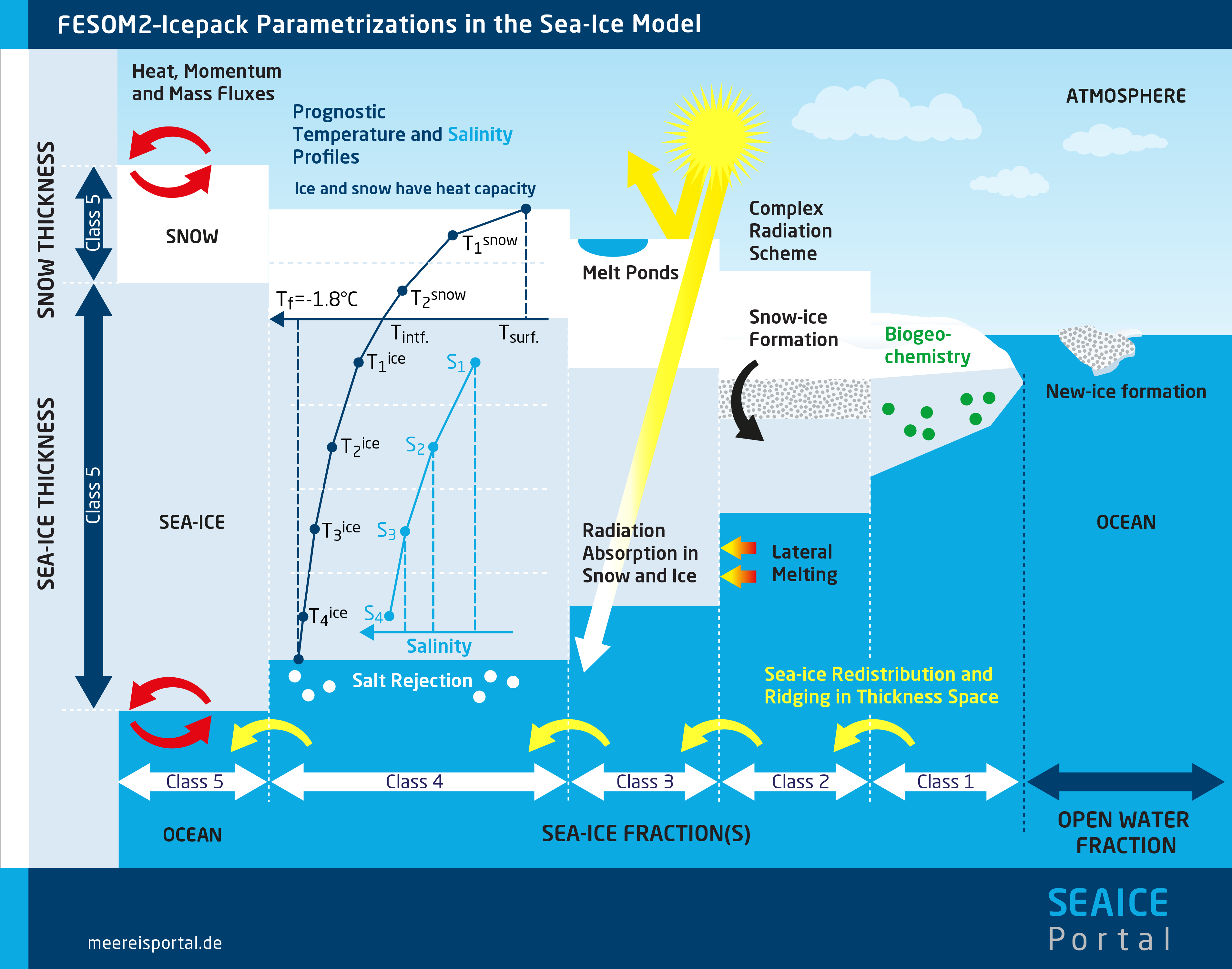
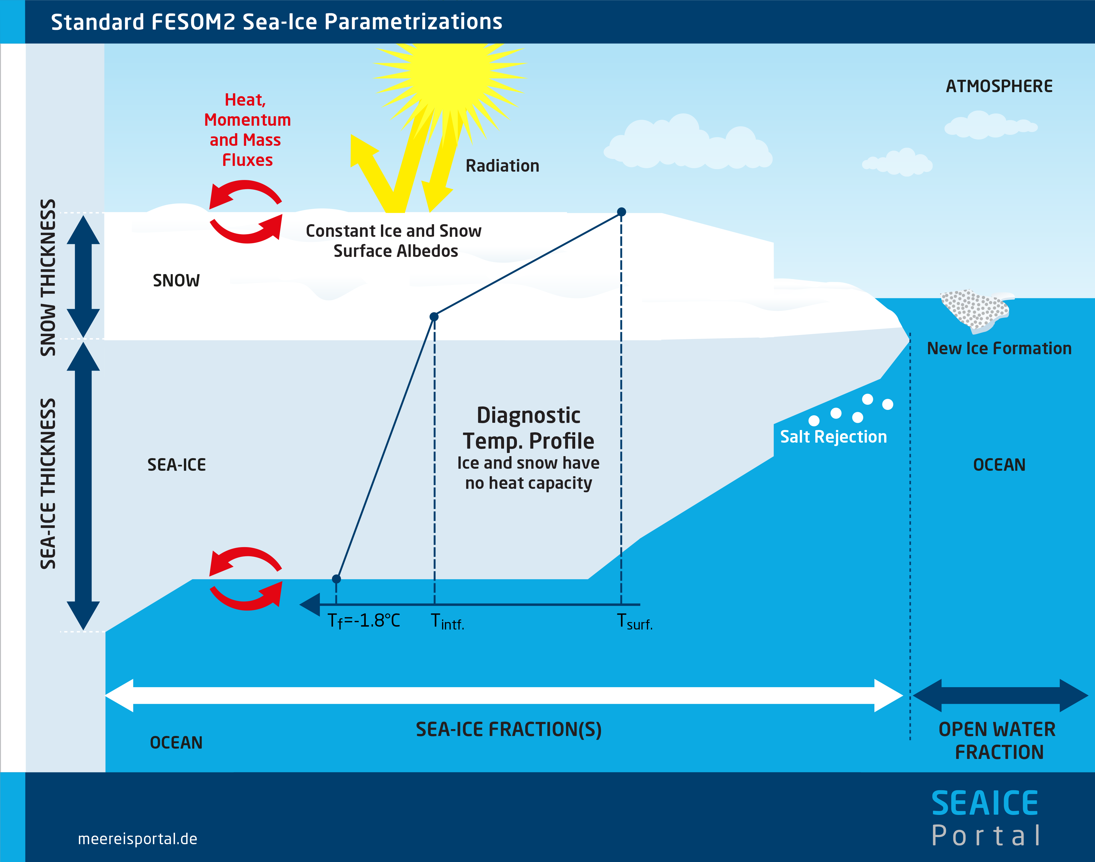
On the one hand, thermodynamic processes affect the respective percentage fractions: additional freezing leads to increased ice thickness, snowfall adds to the depth of the snow cover, and so on. On the other hand, thermodynamic processes can also change the respective fractions. For example, if ice formed in a fraction without sea ice, it would of course no longer be ice-free. In order to avoid this contradiction, the newly formed ice produces a change in the distribution of fractions: the fraction with sea ice expands, at the expense of the ice-free fraction. But in this regard, the devil is in the details. In the following paragraphs, we’ll take a closer look at these details in order to give you an impression of how these processes can be reflected – or parametrised – in sea-ice models.
First, we work under the assumption that the newly formed ice fundamentally has a certain thickness, e.g. half a metre. But we don’t want to add a new fraction just for this new ice; otherwise, the number of fractions would constantly rise. Instead, the newly formed ice is combined with the previous ice fraction. The resulting ice thickness is the mean value of the two fractions, such that the overall increase in ice volume matches the amount of newly formed ice. In this regard, it is quite plausible not to assume that the entire previously ice-free fraction becomes covered with a thin sheet of ice. Rather, in the field it can be observed that, through water and ice movement, ice crystals typically gather at the edges of existing ice floes, where they form new, solid ice.
In complex sea-ice models, various physical and/or biogeochemical processes are also observed in great detail (see figure, left). For example, the sea-ice section is divided into subsections with different ice thicknesses. In this case, new ice formed in the open water initially falls under the thinnest ice-thickness class. The fractions in the respective ice-thickness classes can gradually be transformed into thicker or thinner classes by thermodynamic processes, particularly freezing or melting processes. However, there is also another important type of process that can affect the form of sea ice: motion in which different sections of the ice cover are shoved against one another.
Before taking a look at the influences of motion and other processes, in the following we’ll explain how sea-ice models work using a simple mathematical equation. Here, we won’t go into excessive mathematical detail; but since the physics of the observed processes can only be simulated by computers on the basis of such equations, providing an example would seem to be in order. Changes in sea-ice concentration can be described as follows:
sea-ice concentration (t + 30 minutes) = sea-ice concentration (t) + growth +/- remainder
Therefore, if we know the sea-ice concentration at time t, the equation can tell use the concentration 30 minutes later (t + 30 minutes) by first adding the amount of new ice formed in open water during this time. In this regard, though 30 minutes are only an example, they are also a realistic time interval for a model. Behind this growth lies another equation, one that represents the processes at work in the sea-ice fractions of the grid cells: depending on the temperature of the air that the water (at the freezing point) is in contact with, a certain amount of ice crystals forms. In this regard, we work under the assumption that these ice crystals form a 0.5-metre-thick layer, which in turn allows us to calculate the extent to which the sea-ice concentration increases. Although this assumption is of course a simplification, it has proven its value in the context of modelling. The equation also includes a remainder resulting from other processes, e.g. from ice motion (see “Sea ice in motion” below) or from warmer water producing melting at the edges of the floe.
Needless to say, we need a further equation to describe the development of ice thickness and an equation for each additional parameter; taken together, they describe the ice conditions in the model. On the basis of these equations, the model now proceeds step by step through time, beginning at an initial state that is e.g. derived from observations. In modern global sea-ice and climate models, several equations have to be calculated for millions of grid cells for each time interval. To do so in an acceptable amount of time, supercomputers like those at the German Climate Computing Center (DKRZ) in Hamburg are used.
In addition to temperature-driven (thermodynamic) processes, horizontal motion and shifting affect the ice floes. Taken together, these factors are referred to as sea-ice dynamics. Although dynamics generally refers to force, in this context it describes the ice’s motion and flow behaviour (rheology). Initially, we observe a given grid cell in the sea-ice model, which follows the large-scale motion of the ice. But what happens when winds or ocean currents cause the ice to drift apart? In such situations (referred to as divergence), we can imagine that the areas of open water would simply grow larger.
Things become more complicated when the ice is driven together (convergence). First, the remaining areas of open water may grow smaller: the sea-ice concentration increases. However, once it has nearly reached 100%, it creates stress within the ice that, if the forces are sufficiently strong, can lead floes to stack one on top of the other (rafting). If these forces continue to grow, it can produce fracture zones fault lines in the solid ice cover, where pressure ridges form. Consequently, in the case of convergent ice motion, the sea-ice thickness does not increase homogeneously, but in a highly concentrated form along individual fracture zones. Shearing forces, which can be produced e.g. when sea ice is frozen fast to a coast but is simultaneously driven toward the coast by winds or currents, can also produce ruptures in the ice cover. In turn, these allow the formation of pressure ridges on the one hand and leads of open water on the other.
Simple models with just one ice-thickness class are poorly suited to reflecting such processes, as they only use a mean ice-thickness value. As such, in the event of convergent ice motion, these models can only project what would happen if the thickness increased homogeneously. In contrast, in complex sea-ice models these processes can be accurately reflected by expanding the sections with thick ice and decreasing those with thinner ice classes.
If we observe only the relative motion within a grid cell, the assumption is that the cell will simply follow the large-scale ice motion. However, in order to comprehensively simulate the sea ice and its spatial distribution, this large-scale motion must also be calculated by the model itself. In this regard, essential aspects include the winds and ocean currents, whereas the winds are usually the primary motor and the ocean tends to dampen motion. In models, the forces produced by specific winds or currents are described by means of certain parameters referred to as transfer coefficients. In most cases, it is assumed that the force transferred is proportional to the relative wind or flow speed. As such, twice the relative wind speed produces twice the force.
Because the sea ice, which is usually roughly one to two metres thick, responds quite quickly to these forces, a basic equilibrium of forces is soon reached, an aspect that is also influenced by the Coriolis force and a potential slight tilt in the ocean’s surface. If the direction or intensity of the wind changes, the motion of the ice in the grid cells is correspondingly accelerated, slowed or redirected. But what happens when the ice is driven into an area with a high sea-ice concentration and has nowhere to go, or when the grid cell approaches a coast? Now at the latest, the grid cell can no longer be observed on its own, but must be viewed in connection with its surroundings, e.g. with adjacent cells.
Within a given grid cell, there are forces, stresses and deformation at work on and in the ice. Yet these processes can also have a pronounced effect on large-scale ice motion wherever the sea ice is tightly packed, i.e., where the sea-ice concentration is high. Here, stress within the ice can rapidly produce effects over considerable distances. For example, if the wind drives the ice toward the coast and there are no major leads or other areas of open water in between, the result is stress within the ice, which rapidly passes from grid cell to grid cell and can span several hundred metres. As a result, an internal ice force, which counteracts the force of the wind and keeps the ice in place, is generated across several grid cells.
Accordingly, in areas with a high sea-ice concentration, the forces of wind and water aren’t in equilibrium, as is the case for freely drifting floes. Rather, internal ice stress becomes a crucial factor in the motion equation. And given that this stress can rapidly carry over great distances, the motion equations for several grid cells must be solved simultaneously in models. This has to be done in any case, assuming the goal isn’t to simulate the fate of an individual floe and its immediate surroundings, but the development of the sea ice in a larger context – e.g. for the Arctic or Antarctic as a whole.
There are essentially two strategies for simulating an entire grid consisting of numerous cells. In both variants, the first step is to divide the area in question, e.g. the Arctic, into grid cells of roughly the same size. In the first strategy (“Lagrangian method”), each of the grid cells follows the large-scale ice motion, just as was previously assumed for a single grid cell. The advantage is that the information that can be gleaned e.g. from the ice-thickness distribution is automatically collected over time – with every grid cell, the fate of a specific piece of sea ice is monitored. In contrast, in the second strategy (“Eulerian method”) the simulation points (grid cells) are fixed and the properties of the ice must be transferred from cell to cell, depending on the motion.
The modelling grid that follows the motion of the ice, or Lagrangian approach to sea-ice modelling, is physically elegant, but can entail considerable technical difficulties, as the grid deforms over time, becoming increasingly dense in some areas and increasingly sparse in others (see the linked video in the section From individual grid cells to ocean-wide grids). In regional models, readily apparent problems also arise at the borders of the modelled area. Accordingly, expanding grid cells must be divided and shrinking grid cells must be combined, cells have to be added or removed, and from time to time, all grid cells have to be redefined from scratch. In addition, the data on the condition of the atmosphere and the liquid ocean, which is either interactively calculated with other model components or stems from other datasets, is generally presented on a grid that does not change over time. When the sea-ice grid constantly changes shape, the data points that each individual grid cell has to access have to be constantly recalculated.
Granted, there are also Lagrangian sea-ice models in which the grid follows the motion of the ice (e.g. Rampal et al. 2016). However, it is far simpler, more common and often requires less computing power to define an unchanging grid; this approach is used in virtually every atmospheric and ocean grid model. In fact, the first large-scale sea-ice model that described both the thermodynamics and the dynamics of sea ice applied this “Eulerian” approach, based on a fixed grid (Hibler 1979). This avoids the above-mentioned difficulties. However, it also means bearing in mind that, in response to large-scale motion, the properties of the ice, i.e., the sea-ice concentration etc., are passed from grid cell to grid cell. For example, if the ice drifts from cell A to cell B in the course of a 30-minute interval, so that 10% of cell B now contains ice that was previously in cell A, then in the simplest case, the new status of cell B is the weighted mean of the values for the previous status in the two cells:
Ice status (cell B, time t + 30 minutes) = 90% * ice status (cell B, time t ) + 10 % * ice status (cell A, time t)
In this regard, the “ice status” actually consists of several individual parameters used to describe it in the model: depending on the model’s complexity (see figure), they can include the sea-ice concentration, the percentages for the various thickness classes, the respective snow cover, the temperature and salinity of the ice and snow at various depths, and so on. As such, there are numerous individual equations. And of course, corresponding equations must be provided and solved for cell A and all other cells. Further, it is readily apparent that, in a two-dimensional model, the ice status in several adjacent cells informs these equations, as the figure shows, and the percentages (in the example, 90% and 10%) have to be recalculated at each interval, based on the ice’s current state of motion. Nevertheless, this approach allows advection to be integrated into computer models fairly easily. One disadvantage of the Eulerian method compared to the Lagrangian is that advection gradually leads to numerical diffusion, i.e., to a certain mixing of ice status between the grid cells. Though there are numerical methods that can mitigate this problem of unrealistic mixing, it cannot be eliminated entirely.
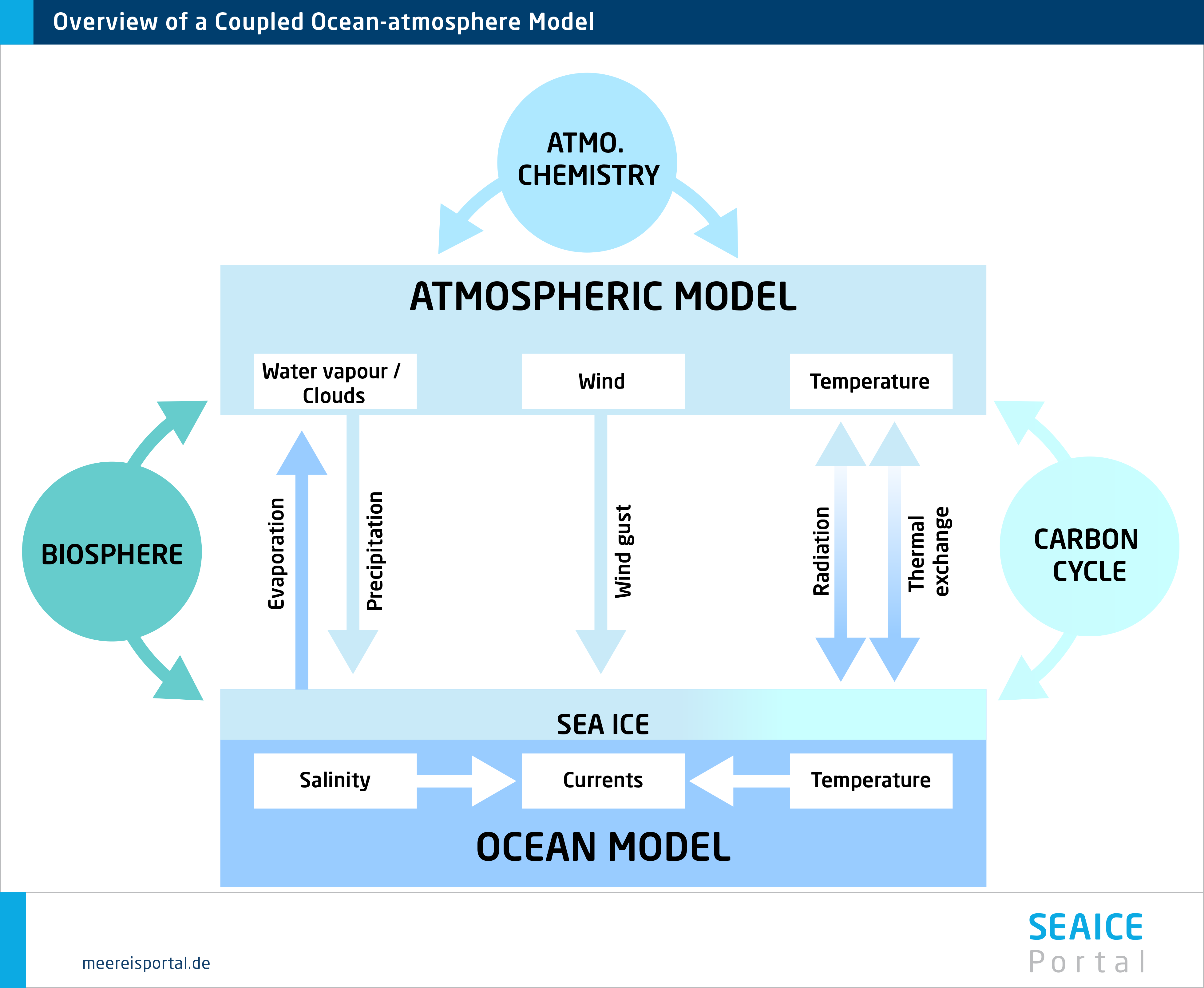
Sea ice as part of the climate system
Sea ice is an important component of the climate system and interacts with the ocean below and atmosphere above in a number of ways. In order to simulate the behaviour of ice over time and how it influences climatic conditions on the Earth as realistically as possible, coupling sea-ice models with models for the ocean and atmosphere is a sensible approach, creating a whole that is greater than the sum of its parts. In the following, we’ll show you how this works.
Sea-ice models describe complex interrelations concerning ice growth and loss, which are affected by thermodynamic and dynamic processes alike. Consequently, they can also be used “uncoupled”, i.e., without further, interactive model components. To do so, the marginal conditions above and below the ice – i.e., the wind, air temperature, incoming radiation and precipitation, as well as the temperature, salinity and currents in the water – together with their development over time must be prescribed on the basis of certain datasets. For the atmosphere, this data is most often taken from what are known as reanalyses, which are routinely produced by operational weather forecasting centres as part of their day-to-day activities, along with weather forecasting models. For the ocean, there are also reanalysis datasets created in a similar manner, i.e., by data assimilation. However, especially in the ice-covered polar regions these datasets are prone to error, as the observational data is particularly lacking.
Another reason why the status of the liquid ocean shouldn’t be prescribed: in order to avoid inconsistencies between the ice status and ocean status. For example, let’s imagine that a large quantity of sea ice drifts into an area characterised by higher water temperatures. In the real world, the ice would begin melting, which would cool the surrounding water and in turn slow the melting rate. In uncoupled sea-ice models, this cooling effect, and therefore also the subsequent slowed melting, is not considered. In contrast, in areas of the oceanic dataset with water temperatures near the freezing point for the high-saline ocean (ca. - 1.8 °C), ice can form as soon as the air temperature drops even lower; if the water temperature is even slightly higher, ice formation is very effectively prevented. As such, the ice distribution simulated in the uncoupled model merely reflects the ice distribution assumed or simulated when the oceanic dataset was created.
Consequently, it is often more sensible, and certainly more common, to couple sea-ice models with equally interactive ocean models. The two component models constantly exchange information on their current status, allowing them to consistently react to one another in keeping with the simulated principles of physics. In many cases, sea-ice models are developed as part of ocean models from the outset, doing away with the need for the external coupling of independent component models. This generally has a practical side-effect: that the two components are described on the same modelling grid, which does away with the need for reconciling two different grids.
Inconsistencies between individual component models in the Earth system can also arise when an ice-ocean model uses prescribed atmospheric data from reanalyses instead of relying on an interactive component model. In fact, these effects can also manifest here – the ice distribution to be simulated is at least partly determined by the pattern of atmospheric temperatures. Nevertheless, there are any number of interesting applications for ice-ocean models.
A further, pressing area in which sea-ice models play an important part: climate change. Here we can see another major limitation of using ice-ocean models without an interactive atmospheric component: the obvious lack of observation-based datasets on the future atmosphere. Accordingly, completely coupled atmosphere-ice-ocean models are called for. In such climate models, the coupling in both directions is very important. Only then can e.g. the amplifying ice-albedo feedback – in which sea-ice retreat caused by warming leads to increased absorption of solar radiation and therefore to further warming – be consistently physically simulated.
Needless to say, climate models (and ice-ocean models) are also used for contexts in which the sea ice is not in focus or is only a secondary consideration. For example, changes in the sea ice aren’t particularly relevant for climate change in the tropics. Nevertheless, in terms of monitoring the climate system from a holistic standpoint, interactive sea-ice models have proven their value as an important element of climate models. In addition, there are indications that changes in the Arctic sea ice may influence the weather in the middle latitudes, including Europe, further underscoring the importance of sea-ice modelling.
In coupled climate models, the sea ice is just one of several important aspects. Whereas the majority of the climate-relevant physics takes place in the atmosphere, the sea ice can – depending on the research focus – be a secondary or essential aspect.
Once it has been determined which equations are to be used in a given sea-ice model, the next step is to define a variety of parameters. For example, one assumption can be that ice crystals forming in open water tend to create a 50-cm-thick layer. But why can’t this parameter – referred to as the lead closing parameter – be 20 centimetre or 1 metre instead?
One might expect that this type of parameter could simply be observed and measured in the field. But in reality, the ice formation process can vary considerably. This in turn depends on a number of factors – e.g. the wave action, width of the lead, and temperature – and in a complex manner, making it very difficult to measure. One could attempt to include these complex interdependencies by integrating additional equations and parameters into the model. However, most often these new equations would also involve new parameters that are equally difficult to measure.
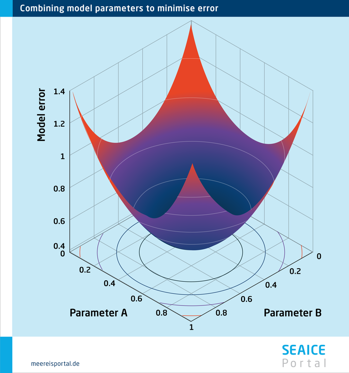
Accordingly, at a certain point, modellers have to accept a certain amount of remaining imprecision and prescribe values for the uncertain parameters. This involves a degree of estimation and is true not just for the lead closing parameter, but for many other parameters, e.g. those that determine at which level of stress cracks begin to form in the ice, or how the redistribution from thinner to thicker ice classes progresses during the formation of pressure ridges. But necessity can be made the mother of invention, namely by making the selected parameters dependent on how realistic the resulting simulations are. Here, properties for which comparatively precise and comprehensive observations are available can be used for guidance. In the case of sea ice, the changing position of the ice edge through the seasons is particularly well suited. Other observable parameters that are commonly used include large-scale ice-thickness and ice-drift patterns.
This is referred to as model tuning, and the uncertain parameters involved are called tuning parameters. Whether this is done manually, i.e., by trying out different combinations of parameters one at a time, relying on experience and, to some extent, instinct; or whether the optimisation process is automated or handled more objectively, is up to the individual researcher. In fact, to this day, (at least partially) manual approaches are more common in climate research, since automated approaches require considerable computing power and don’t always deliver the desired degree of objectivity. One example in which the comparatively objective tuning of sea-ice models was used very successfully can be found in the study by Zampieri et al. (2021).
Due to their nature, sea-ice models and climate models include simplified equations and uncertain parameters, making it necessary to optimise (tune) them. If, even after painstaking tuning, a given model does not reflect key aspects of the reality – like the seasonal development of Arctic sea-ice extent – then the model is manifestly not yet “good” and, if possible, its equations need to be further refined.
That being said, not every successfully tuned model is automatically a good one. For example, a given model might very accurately reproduce those observations used for tuning but display considerable model error when new observations are used for comparison. This can be the result of overfitting and becomes more likely, the more uncertain tuning parameters the model contains, and the fewer observations are used in the tuning. In this case, there can be any number of parameter combinations that ostensibly perform well in the tuning.
As such, it is fundamentally advisable to use as many observations as possible for tuning. This applies not just to the spatiotemporal scope of the observations, but also to reflecting the most important parameters (e.g. ice concentration, thickness and drift) and to including as many as possible of the status types that the model is meant to simulate. For example, if a sea-ice model (whether coupled or uncoupled) is to be used for short-term sea-ice predictions, it can be helpful for the observations to include a wide variety of unusual events, to ensure that they, too, can be realistically simulated. However, it should also be kept in mind that satellite observations in particular aren’t error-free, which can lead to inconsistencies between the observations of different parameters, making the tuning even more difficult.
When it comes to long-term climate projections, the last criterion – including as many as possible of the status types that the model is meant to simulate in the tuning – is essentially impossible to fulfil. Accordingly, in such applications it is all the more important that there are as few uncertain tuning parameters as possible. This in turn means basing the model’s equations on the bedrock of fundamental physics as much as possible, instead of making them dependent on parametrisations. As such, the rule of thumb is the old adage, attributed to Einstein, that everything should be made as simple as possible, but not simpler. In this regard, how complex a given model has to be depends on the respective application it is intended for; after all, the key aspects required for the research question at hand have to be included.
In practice, it’s not always possible to replace uncertain parametrisations with fundamental physical equations. Consequently, a remainder of model-based uncertainty is unavoidable, in short-term sea-ice forecasts and long-term climate and sea-ice projections alike. However, there are promising approaches designed to refine models, making them more and more “physical” and thus less uncertain. They can be broken down into three fundamental directions.
- There are new observations, stemming e.g. from the MOSAiC expedition or new satellite or aerial missions, that can be very important. In this way, processes can be more fully understood and better – more physical – parametrisations can be developed. New field data like that gathered during the MOSAiC expedition offers an important basis for the continuing development of sea-ice models.
- As (super)computers become more powerful, it is becoming possible to use higher and higher spatial resolution, i.e., smaller and smaller grid cells. As a result, more and more of e.g. the ice-thickness distribution, ice stress and motion can now be explicitly simulated; uncertain parametrisations are becoming less relevant.
Interestingly, over the past few years it has become apparent that structures in the sea ice – in particular, large leads – appear at resolutions below ca. 5 km, even though the dynamic equations borrowed from lower-resolution models aren’t actually designed to reflect such structures. Exploring such phenomena and how models’ equations can be optimised for higher resolutions is a highly active field of research in sea-ice modelling. - Fundamentally speaking, researchers’ ingenuity is also a vital aspect: new ideas can lead to better models without the need for additional observations or faster computers, e.g. through new parametrisations or innovations in numerical methods.
Box, G. (1979): Robustness in the Strategy of Scientific Model Building, in: Robustness in Statistics, edited by LAUNER, R. L. and WILKINSON, G. N., pp. 201–236, Academic Press. doi.org/10.1016/B978-0-12-438150-6.50018-2
Hibler, W. D. (1979): A dynamic thermodynamic sea ice model. Journal of physical oceanography, 9(4), 815-846.
Rampal, P., Bouillon, S., Ólason, E., & Morlighem, M. (2016): neXtSIM: a new Lagrangian sea ice model. The Cryosphere, 10(3), 1055-1073.
Zampieri, L., Kauker, F., Fröhle, J., Sumata, H., Hunke, E. C., & Goessling, H. F. (2021): Impact of sea‐ice model complexity on the performance of an unstructured‐mesh sea‐ice/ocean model under different atmospheric forcings. Journal of Advances in Modelling Earth Systems, 13, e2020MS002438. doi.org/10.1029/2020MS002438